Physical Neural Networks - The Harmonic Oscillator, Part I

I’ve been really interested in machine learning and neural networks in the context of physics recently. When I came across Ben Moseley’s post on Physics Informed Neural Networks, I instantly knew what I was going to be doing this afternoon – I wanted to implement neural networks using Mathematica to solve a simple problem, the Harmonic Oscillator. As Sidney Coleman once said,

“The career of a young theoretical physicist consists of treating the harmonic oscillator in ever-increasing levels of abstraction,”

and applying sufficiently well trained neural network to a canonical problem in physics is well within the limits of abstraction.

Theory #

The canonical problem of the harmonic oscillator is to understand a system with a restoring force \(F(\chi)=-k\chi.\) For a single restoring force acting on masses connected to springs, or pendulums freely moving in a gravitational field, the system undergoes simple harmonic motion induced by the restoring force. Mathematically, the objective is to solve the system:

$$ \begin{equation*}m\frac{d^2\chi(t)}{dt^2} + k\chi(t)=0\end{equation*} $$

subject to some initial data \((\chi(0)=\xi,\chi’(0)=\zeta)\). Of course, any budding physicist knows there is an exact solution

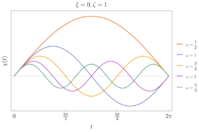
$$\begin{equation*}\chi(t) = \frac{\zeta}{\omega}\sin(\omega t) + \xi\cos(\omega t)\end{equation*}$$

which has a straightforward wave-like behavior plotted below for a representative set of solutions.

Applications #

Now, we turn to the problem of constructing neural networks with Mathematica architecture in order to learn harmonic motion directly. We will train the network for the parameters and the domain

$$\begin{equation*}[\xi=1,\zeta=0,\omega=3;\ t_{\rm sample}\in(0,\pi)]\end{equation*}$$

Mathematica’s neural network algorithms can produce a trained fit to the initial sample. Here, I show how I did it but more documentation can be found in this post.

The algorithm is as follows. First, construct the solution with the parameters above. I created a function Sols which solves the differential equation for harmonic motion provided data $(\xi,\zeta,\omega)$. For this particular example, I created an instance

Oscillator[t_] := Evaluate[Sols[t, 1, 0, 3]];

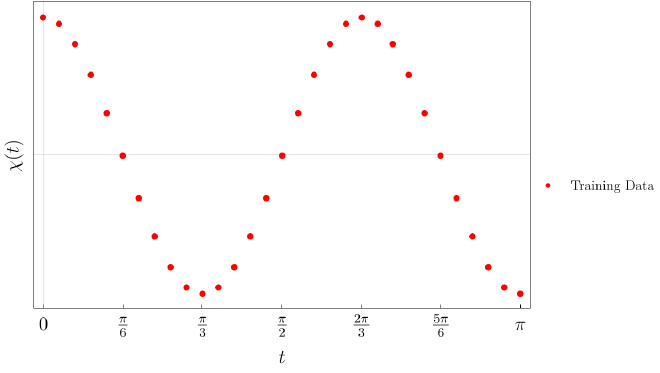
Next, gather some training data. I chose about 30 points to train the neural network (NN).

data = Simplify[
   Table[t -> Oscillator[t], {t, 0, \[Pi], \[Pi]/30}] // N];

Now, construct a neural network with NetChain. I chose a NN with 5 hidden layers, and 1 input/output layer respectively. The model uses different types of ElementwiseLayer, such as IntegerParts, Tanh, and LogisticSigmoid, to train the network. I found that this was best for convergence.

net = NetChain[{150, Tanh, 150, LogisticSigmoid, 1}]

The five entries provided in NetChain define functions only on the hidden layer. Finally, we can train the model with NetTrain.

trainingdata = NetTrain[net, data, All, TimeGoal -> 30]

Essentially, this takes the NN and trains it on the sample data in around 30 seconds. The NN converged rather quickly to a loss of about $3.67\times 10^{-5}$.

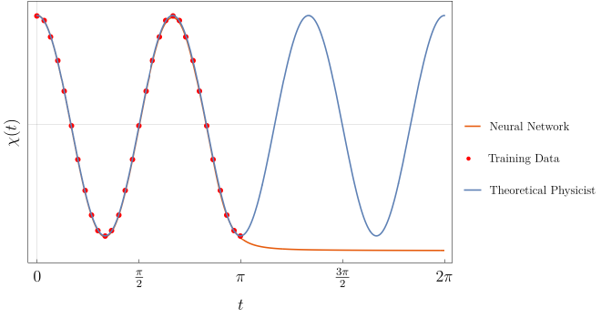
And we’re done! Let’s visualize the trained data now, the results are shown in the plot below.

Although the neural networks performs a good fit when trained, it has not learned any physics in any meaningful way. So for now, it seems a young theoretical physicist can still beat a well trained neural network. But this result brings up a natural question, can we do better using Mathematica architecture?

It turns out the answer is no, see here for a more extensive discussion.

The goal of Part II is to reproduce Ben’s calculation in Physics-Informed Neural Networks by writing better neural networks which incorporates a regularization scheme where the equation of motion is simultaneously minimized along with a cost function.