Computing the Entanglement Entropy with the Quantum Framework Paclet

The entanglement entropy is a measure of how quantum information is stored in a quantum state. In particular, the entanglement entropy measures the amount of entanglement between two subsystems of a composite quantum system. Here, I will review the entanglement entropy and then compute it for a simple example – the two spin system both analytically and with the QuantumFramework Packlet on Mathematica 13. I will largely be following Nishioka 2018, Hong Liu’s HEE MIT lecture, and Tom Hartman’s excellent notes.

Theory #

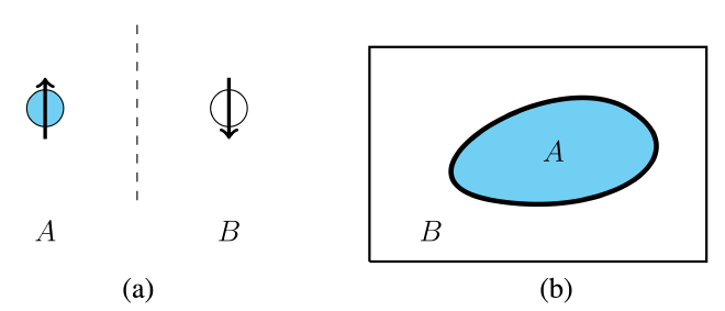
The canonical example is to consider a system which is subdivided into two regions $A$ and $B$, see figure below taken from Nishioka 2018.

The system $\Sigma$ is said to be bipartite if its Hilbert space $\mathcal{H}_ \Sigma$ can be expressed by the tensor product $$ \mathcal{H}_ \Sigma = \mathcal{H}_ I\otimes\mathcal{H}_ {I^c} $$ over the individual subsystems where $I=A$ or $B$. To see if the two subsystems are entangled, we need further technologies: a density matrix $\rho_ \Sigma$ and an operation $\text{Tr}_ I$ which isolates a subsystem. The first is easy, the density matrix, by definition, is constructed from the (pure) quantum state $\ket{\Psi}\in\mathcal{H}_ \Sigma$ of the system

$$\begin{equation*}\rho_ \Sigma = \ket{\Psi}\bra{\Psi}.\end{equation*}$$

For the second, let ${\ket{i}_ I, i=1,2,\cdots, \dim(\mathcal{H}_ I)}$ be an orthonormal basis for $\mathcal{H}_ I$. The partial trace $ \text{Tr}_ {I}$ of an operator $\mathcal{O}$ is then defined by

$$\begin{equation*}\text{Tr}_ I(\mathcal{O}) \equiv \sum_ {i} {}_ {I}\bra{i}\mathcal{O}\ket{i}_ {I}.\end{equation*}$$

The partial trace can be used to isolate a subsystem $I$ by “tracing out” the complement $I^c$. To be concrete, the reduced density matrix of the subsystem $I$ is obtained via

$$\begin{equation*}\rho_ {I} \equiv \text{Tr}_ {I^c}(\rho_ \Sigma).\end{equation*}$$

We now have the necessary ingredients to compute the von Neumann entropy stored in the entanglement between $I$ and $I^c$. The entanglement entropy of the subsystem $I$ is computed by the formula

$$\begin{equation*}S_ I = - \text{Tr}_ {I}[\rho_ {I}\log(\rho_ {I})].\end{equation*}$$

This entropy satisfies the following statements:

1. The entanglement entropy is non-zero only if the complement of the subsystem is non-empty. In other words, $S_ I=0$ when $\text{Area}(I^c)=0$. To see this, first note that $\text{Area}(I^c)=0$ is the same as saying $I^c=\emptyset$. Next, we have $\Sigma = I \cup I^c = I \cup \emptyset = I$. And finally, it is well known that the entanglement entropy of the total system always vanishes for a pure state. Proof: $$\begin{align*}S_ I &= - \text{Tr}_ {I}[\rho_ {I}\log(\rho_ {I})] = - \text{Tr}_ {\Sigma}[\rho_ \Sigma\log(\rho_ \Sigma)] = - \text{Tr}_ {\Sigma}[ODO^{-1}\log(ODO^{-1})]\newline&=-\text{Tr}_ {\Sigma}[D\log(D)]=0\end{align*}$$ where we have used that the density matrix (i) can be diagonalized, i.e., $$\rho_{\Sigma}=ODO^{-1}$$ and (ii) the ground state is pure so $$\rho_\Sigma = (\rho_\Sigma)^2$$ implying that the eigenvalues $\lambda_i\in{0,1}.$

2. The entanglement entropy is finite for finite-dimensional quantum systems, such as on a lattice. However, $S_I$ suffers from UV divergences in quantum field theory (necessarily infinite dimensional) due to short range interactions near the boundary of $I$, denoted $\partial I$.

3. It is possible to show that the entanglement entropy vanishes only if the pure ground state is separable which means that the quantum state admits the decomposition $\ket{\Psi} = \ket{\Psi}_ I\otimes\ket{\Psi}_ {I^c}$. In the case where $\text{Area}(I^c)=0$, there exists no states in $\mathcal{H}_ {I^c}$ and hence the bipartition is simple $\ket{\Psi}=\ket{\Psi}_ I\otimes 1 = \ket{\Psi}_ \Sigma$.

Applications #

This is all well and good in theory, but how does one actually go about computing the entanglement entropy given a state?

The simplest example is the two spin system (see Fig. 1(a)). Let $A$ and $B$ be two particles with spin $s=1/2$. Each particle has two states in their respective Hilbert spaces $$H_ {I}=\text{span}({\ket{\uparrow}_ I,\ket{\downarrow}_ I})$$ where $I=A$ or $B$ and the bases are orthonormal $\braket{i}{j}=\delta_{ij}$ for $i,j\in{\uparrow,\downarrow}$. The total Hilbert space is then straightforward to build $$\mathcal{H}_ \Sigma =\mathcal{H}_ I\otimes\mathcal{H}_ {I^c}= {\ket{\downarrow\downarrow},\ket{\downarrow\uparrow},\ket{\uparrow\downarrow},\ket{\uparrow\uparrow}}$$ where $\ket{ij}\equiv\ket{i}_ I\otimes\ket{j}_ {I^c}$.

Now, suppose the ground state is given as

$$\begin{equation*}\ket{\Psi} = \frac{1}{\sqrt{2}}(\ket{\downarrow\uparrow}+\ket{\uparrow\downarrow})\end{equation*}$$

then the density matrix of the total system reads

$$\begin{equation*}\rho_\Sigma=\ket{\Psi}\bra{\Psi}=\frac{1}{2}(\ket{\downarrow\uparrow}+\ket{\uparrow\downarrow})^2.\end{equation*}$$

Tracing out, say $I^c=B$, we arrive at the reduced density matrix for $I=A$

$$\begin{align*}\rho_A = \frac{1}{2}(\ket{\downarrow}_A{}_A\bra{\downarrow}+\ket{\uparrow}_A{}_A\bra{\uparrow}) = \begin{pmatrix}1/2 & 0\newline0 &1/2\end{pmatrix} \end{align*}$$

And now a straightforward calculation of the entanglement entropy $S_A$ shows

$$\begin{align*}S_{A} &= -\text{Tr}_A\left[\begin{pmatrix}1/2 & 0\newline0 &1/2\end{pmatrix}\cdot\begin{pmatrix}\log(1/2) & 0\newline0 &\log(1/2)\end{pmatrix}\right]\newline&=\log(2)\end{align*}$$

This seemingly innocous value is in fact the maximum amount of von Neumann entropy (or more loosely information) stored between two entangled particles! To prove this statement, let us consider a more general state

$$\ket{\Psi} = \cos(\theta)\ket{\downarrow\uparrow}-\sin(\theta)\ket{\uparrow\downarrow}$$

and study this problem in Mathematica 13.

Entanglement Entropy on Mathematica 13 #

Recently, the Quantum Information Research Team at Wolfram Alpha have developed frameworks which greatly simplify the calculations required to compute the entanglement entropy (in low dimensional examples). This code can be found on my Github.

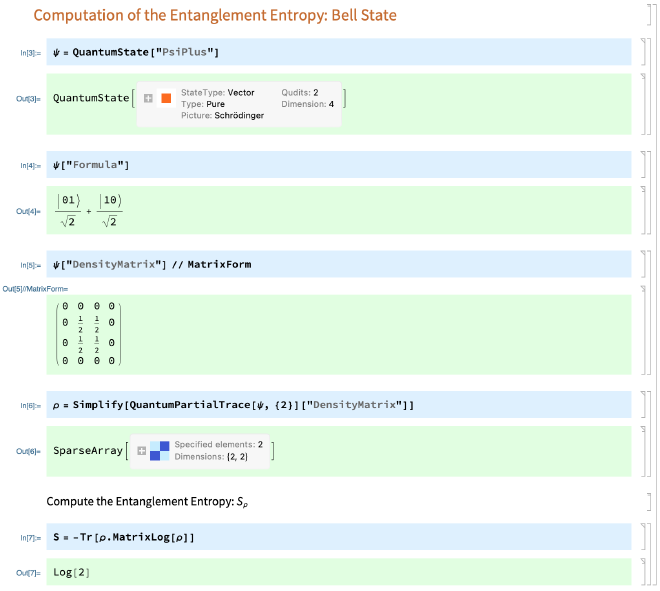
The code snippet below demonstrates how the QuantumFramework packlet can be used to reproduce the entanglement entropy of the Bell state.

Now to study the generalized Bell state, we essentially reproduce the code but have to change the initial state:

Hence, the entanglement entropy stored in the generalized entangled states is

$$S_A(\theta) = -2\left[\cos(\theta)^2\log(\cos(\theta))+\sin(\theta)^2\log(\sin(\theta)) \right]$$

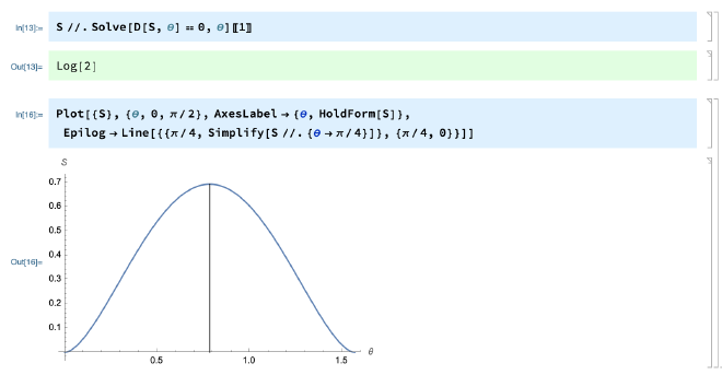
Now, we are ready to maximize $S_A(\theta)$ and prove that $S_A=\log(2)$ is the maximum amount of entropy which can be stored in two-spin system. This amounts to finding $\theta_c$ such that $$\frac{d}{d\theta}S_A(\theta)\rvert_{\theta_c}=0.$$ A quick calculation shows

$$\theta_c = \frac{\pi}{4} \implies S_{A}(\theta_c) = \log(2).$$

It is also immediate to show this on Mathematica:

The purpose of this post was to discuss some basic facts about the entropy of entanglement and study a simple example both analyticially and numerically. In a future post, we study the case of the Thermofield double state as we slowly build towards the holographic entanglement entropy.

Acknowledgments #

I appreciate Å. Folkestad for comments.